SPAGxEmix_CCT-local

SPAGxEmix_CCT-local is a scalable and accurate G×E analysis framework that allows tests for ancestry-specific effects by incorporating local ancestry in multi-way admixed populations.

Introduction of SPAGxEmix_CCT-local

SPAGxEmix_CCT-local extends SPAGxEmix_CCT by integrating local ancestry information to enhance the precision of ancestry-specific G×E effect testing and statistical powers. Furthermore, we introduce SPAGxEmix_{CCT-local-global}, which combines p-values from both SPAGxEmix_CCT and SPAGxEmix_CCT-local, offering an optimal unified approach for various cross-ancestry genetic architectures. As with SPAGxEmix_CCT, SPAGxEmix_CCT-local involves two main steps:

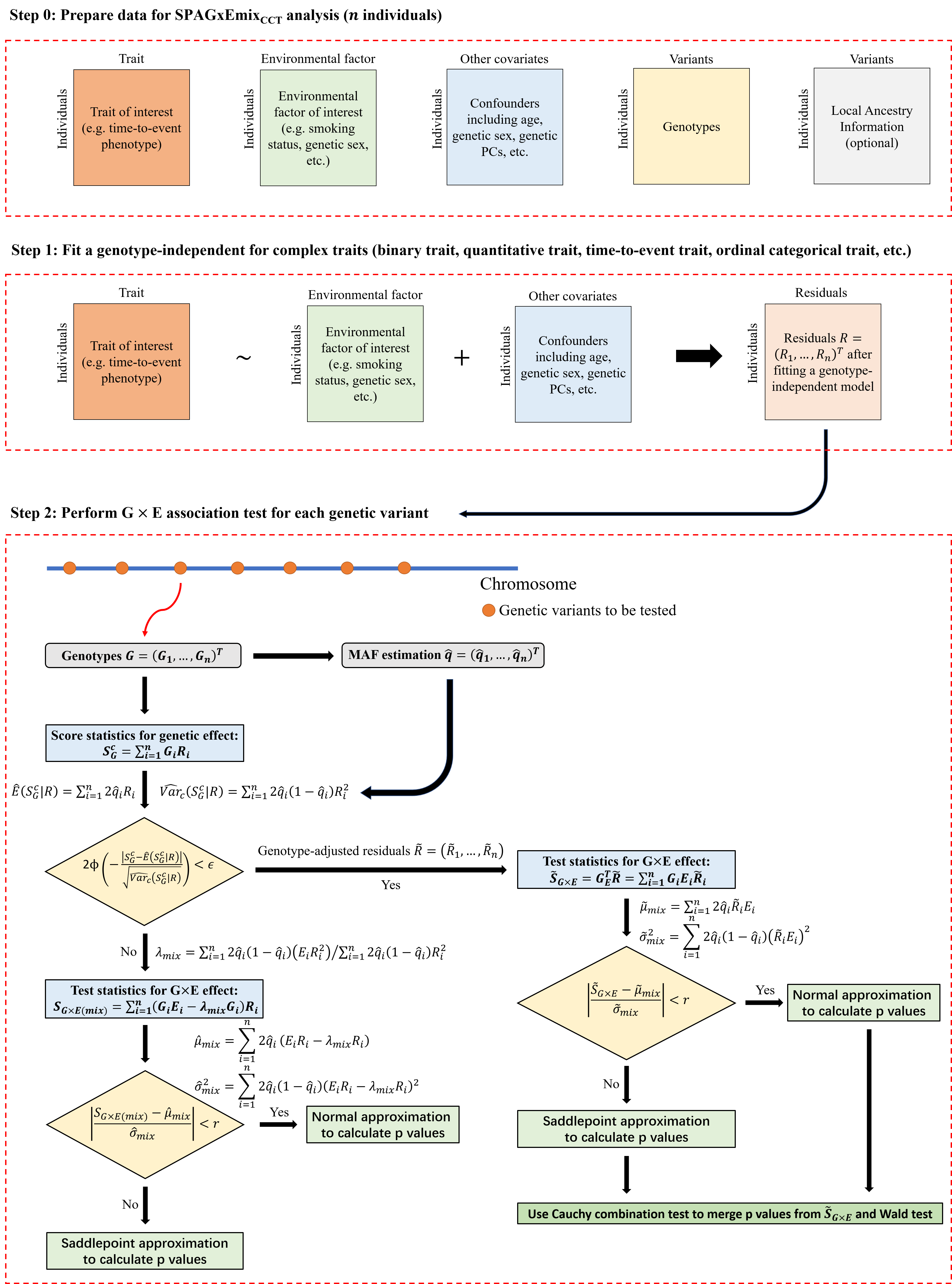
• Step 1: SPAGxEmix_CCT-local fits a genotype-independent (covariates-only) model and calculates the model residuals. Details are described in Step 1 of SPAGxE_CCT.

• Step 2: SPAGxEmix_CCT-local identifies genetic variants with marginal G×E effects on the trait of interest. First, SPAGxEmix_CCT-local estimates the ancestry-specific allele frequencies for the variants. Next, SPAGxEmix_CCT-local evaluates ancestry-specific marginal genetic effects using ancestry-specific score statistics. If an ancestry-specific marginal genetic effect is not significant, we use ancestry-specific test statistic S_G×E(mix) to characterize the ancestry-specific marginal G×E effect. If significant, S_G×E(mix) is updated to ancestry-specific genotype-adjusted test statistics. The hybrid strategy to balance computational efficiency and accuracy follows SPAGxE_CCT.

Compared to conventional standard statistical testing methods that account for local ancestry, SPAGxEmix_CCT-local offers much greater computational efficiency.

• SPAGxEmix_CCT-local leverages local ancestry information to estimate the distribution of ancestry-specific genotypes and the null distribution of test statistics.
• For most tests (ancestry-specific genetic main effect p-values > 0.001) in a genome-wide G×E analysis, SPAGxEmix_CCT-local utilizes residuals from a genotype-independent model (fitted only once across the genome-wide analysis) to construct test statistics.
• Conventional methods have to incorporate local ancestry as covariates and fit a separate model for each variant, which is computationally burdensome for genome-wide analyses.

Quick start-up examples

The following example illustrates how to use SPAGxEmix_CCT-local to analyze a binary trait.

Step 1. Read in data and fit a genotype-independent model

library(SPAGxECCT)
# load in phenotype, genotype, and local ancestry counts for two ancestries
data("Pheno.mtx")           # phenotype data
data("Geno.mtx")            # genotype data
data("Geno.mtx.ance1")      # ancestry-specific genotype data for ancestry 1
data("Geno.mtx.ance2")      # ancestry-specific genotype data for ancestry 2
data("haplo.mtx.ance1")     # local ancestry counts for ancestry 1
data("haplo.mtx.ance2")     # local ancestry counts for ancestry 2

Cova.mtx = Pheno.mtx[,c("PC1", "PC2", "PC3", "PC4", "Cov1", "Cov2")]   # Covariate matrix excluding environmental factor
E = Pheno.mtx$E                                                        # environmental factor

### Cova.haplo.mtx.list
Cova.haplo.mtx.list = list(haplo.mtx.ance1 = haplo.mtx.ance1,
                           haplo.mtx.ance2 = haplo.mtx.ance2) # local ancestry counts of ancestry 1 and 2

### fit a genotype-independent model for the SPAGxEmix_CCT_local analysis
resid  = SPA_G_Get_Resid(traits = "binary",
                         y ~ Cov1 + Cov2  + E + PC1 + PC2 + PC3 + PC4,family=binomial(link="logit"),
                         data = Pheno.mtx,
                         pIDs = Pheno.mtx$IID,
                         gIDs = rownames(Geno.mtx))

Step 2. Conduct a marker-level association study

### calculate p values for ancestry-specific GxE effects of ancestry 1
binary_res_ance1 = SPAGxEmixCCT_localance(traits = "binary",
                                          Geno.mtx = Geno.mtx.ance1,
                                          R = resid,
                                          haplo.mtx = haplo.mtx.ance1,
                                          E = E,
                                          Phen.mtx = Pheno.mtx,
                                          Cova.mtx = Cova.mtx,
                                          Cova.haplo.mtx.list = Cova.haplo.mtx.list)

colnames(binary_res_ance1) = c("Marker", "MAF.ance1","missing.rate.ance1",
                               "Pvalue.spaGxE.ance1","Pvalue.spaGxE.Wald.ance1", "Pvalue.spaGxE.CCT.Wald.ance1",
                               "Pvalue.normGxE.ance1", "Pvalue.betaG.ance1",
                               "Stat.betaG.ance1","Var.betaG.ance1","z.betaG.ance1")

### calculate p values for ancestry-specific GxE effects of ancestry 2
binary_res_ance2 = SPAGxEmixCCT_localance(traits = "binary",
                                          Geno.mtx = Geno.mtx.ance2,
                                          R = resid,
                                          haplo.mtx = haplo.mtx.ance2,
                                          E = E,
                                          Phen.mtx = Pheno.mtx,
                                          Cova.mtx = Cova.mtx,
                                          Cova.haplo.mtx.list = Cova.haplo.mtx.list)

colnames(binary_res_ance2) = c("Marker", "MAF.ance2","missing.rate.ance2",
                               "Pvalue.spaGxE.ance2","Pvalue.spaGxE.Wald.ance2", "Pvalue.spaGxE.CCT.Wald.ance2",
                               "Pvalue.normGxE.ance2", "Pvalue.betaG.ance2",
                               "Stat.betaG.ance2","Var.betaG.ance2","z.betaG.ance2")

### merge data frame
binary.res = merge(binary_res_ance1, binary_res_ance2)

# we recommand using column of 'p.value.spaGxE.CCT.Wald.index.ance' to associate genotype with phenotypes
head(binary.res)

Citation

• A scalable and accurate framework for large-scale genome-wide gene-environment interaction analysis and its application to time-to-event and ordinal categorical traits (to be updated).