SPAGxEmixCCT
As an extension of SPAGxECCT, SPAGxEmixCCT is a G×E analytical framework which is applicable to individuals from multiple ancestries or multi-way admixed populations.
Introduction of SPAGxEmixCCT
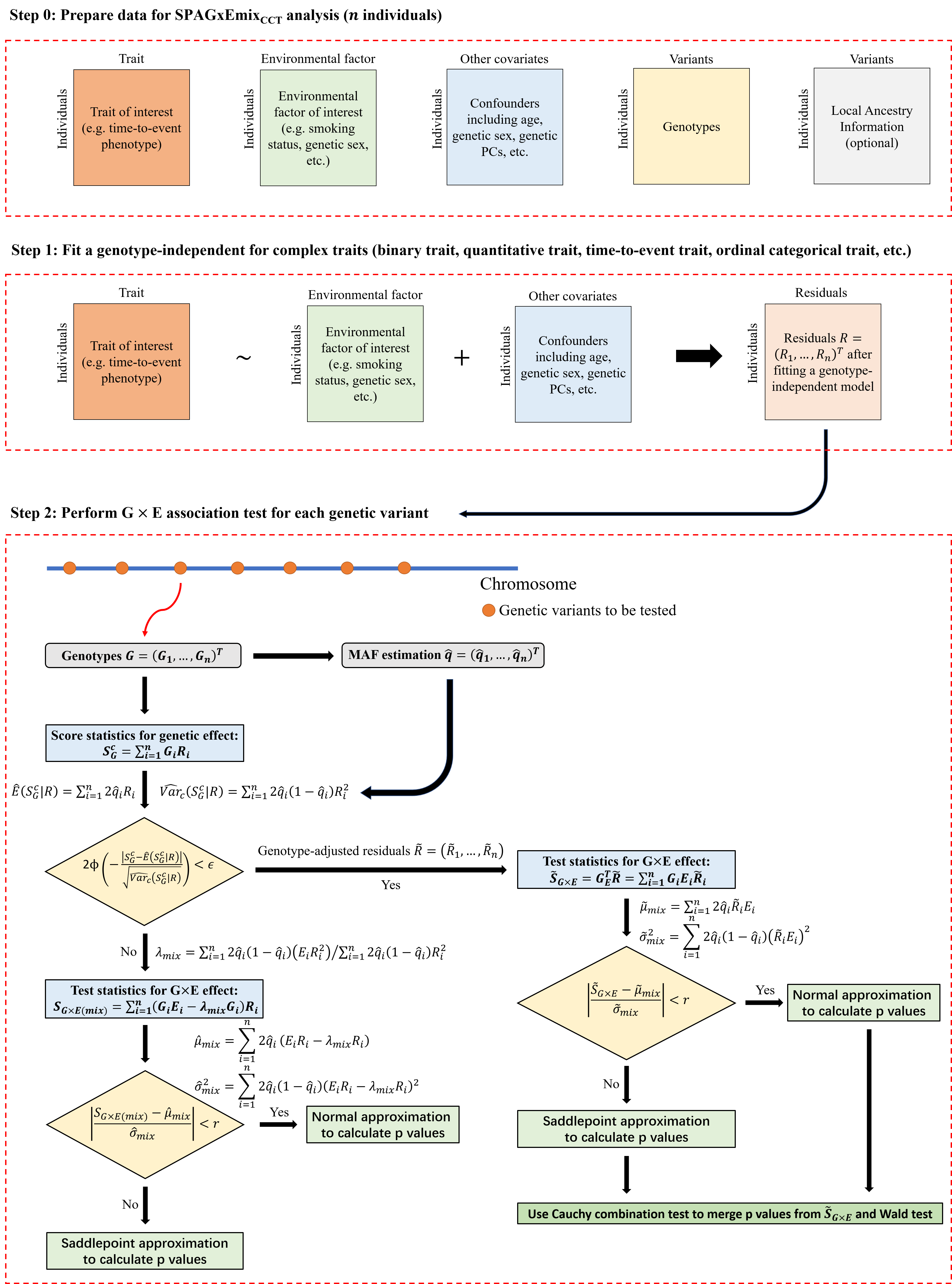
SPAGxEmixCCT allows for different allele frequencies for genotypes. SPAGxEmixCCT estimates individual-level allele frequencies using SNP-derived principal components (PCs) and raw genotypes. Similar to SPAGxECCT, SPAGxEmixCCT involves two main steps:
-
Step 1: SPAGxEmixCCT fits a genotype-independent (covariates-only) model and calculates the model residuals. Detailed information is provided in Step 1 of SPAGxECCT.
-
Step 2: SPAGxEmixCCT identifies genetic variants with marginal G×E effects on the trait of interest. It first estimates the individual-level allele frequencies of the tested variants using SNP-derived PCs and raw genotypes. Next, SPAGxEmixCCT evaluates marginal genetic effects using score statistics. If the marginal genetic effect is not significant, SG×E(mix) is used as the test statistic to characterize the marginal G×E effect. If significant, SG×E(mix) is updated to genotype-adjusted test statistics. The hybrid strategy to balance computational efficiency and accuracy follows SPAGxECCT.
Main features of SPAGxEmixCCT
Admixed populations are routinely excluded from genomic studies due to concerns over population structure. The admixed population analysis is technically challenging as it requires addressing the complicated patterns of genetic and phenotypic diversities that arise from distinct genetic backgrounds and environmental exposures. As the genetic ancestries are increasingly recognized as continuous rather than discrete, SPAGxEmixCCT estimates individual-level allele frequencies to characterize the individual-level genetic ancestries using information from the SNP-derived PCs and raw genotype data in a model-free approach.
-
SPAGxEmixCCT does not necessitate accurate specification of and the availability of appropriate reference population panels for the ancestries contributing to the individual, which might be unknown or not well defined.
-
SPAGxEmixCCT is not sensitive to model misspecification (e.g. missed or biased confounder-trait associations) and trait-based ascertainment.
Quick start-up examples (genotype input using R matrix format)
The following example illustrates how to use SPAGxEmixCCT to analyze a time-to-event trait, with genotype data input provided in the R matrix format.
Step 1. Read in data and fit a genotype-independent model
library(SPAGxECCT)
# Simulate phenotype and genotype
N = 10000
N.population1 = N/2
N.population2 = N/2
nSNP = 100
MAF.population1 = 0.1
MAF.population2 = 0.3

Geno.mtx.population1 = matrix(rbinom(N.population1*nSNP,2,MAF.population1),N.population1,nSNP)
Geno.mtx.population2 = matrix(rbinom(N.population2*nSNP,2,MAF.population2),N.population2,nSNP)
Geno.mtx = rbind(Geno.mtx.population1, Geno.mtx.population2)
# NOTE: The row and column names of genotype matrix are required.
rownames(Geno.mtx) = paste0("IID-",1:N)
colnames(Geno.mtx) = paste0("SNP-",1:nSNP)

Phen.mtx.population1 = data.frame(ID = paste0("IID-",1:N.population1),
                                  event = rbinom(N.population1,1,0.5),
                                  surv.time = runif(N.population1),
                                  Cov1 = rnorm(N.population1),
                                  Cov2 = rbinom(N.population1,1,0.5),
                                  E = rnorm(N.population1),
                                  PC1 = 1)

Phen.mtx.population2 = data.frame(ID = paste0("IID-",(N.population1+1):N),
                                  event = rbinom(N.population2,1,0.5),
                                  surv.time = runif(N.population2),
                                  Cov1 = rnorm(N.population2),
                                  Cov2 = rbinom(N.population2,1,0.5),
                                  E = rnorm(N.population2),
                                  PC1 = 0)

Phen.mtx = rbind.data.frame(Phen.mtx.population1,
                            Phen.mtx.population2)   # phenotype dataframe
E = Phen.mtx$E                                      # environmental factor
Cova.mtx = Phen.mtx[,c("Cov1","Cov2", "PC1")]       # Covariate matrix excluding environmental factor

# Attach the survival package so that we can use its function Surv()
library(survival)

### fit a genotype-independent model for the SPAGxEmix_CCT analysis
R = SPA_G_Get_Resid("survival",
                    Surv(surv.time,event)~Cov1+Cov2+PC1+E,
                    data=Phen.mtx,
                    pIDs=Phen.mtx$ID,
                    gIDs=paste0("IID-",1:N))
Step 2. Conduct a marker-level association study
# calculate p values
survival.res = SPAGxEmix_CCT(traits = "survival",                     # trait type
                             Geno.mtx = Geno.mtx,                     # genotype vector
                             R = R,                                   # residuals from genotype-independent model
                             E = E,                                   # environmental factor
                             Phen.mtx = Phen.mtx,                     # phenotype dataframe
                             Cova.mtx = Cova.mtx,                     # Covariate matrix excluding environmental factor
                             topPCs = Cova.mtx[,"PC1"])               # SNP-derived top PCs

# we recommand using column of 'p.value.spaGxE.CCT.Wald' to associate genotype with time-to-event phenotypes
head(survival.res)
Quick start-up examples (genotype input using PLINK file format)
The following example illustrates how to use SPAGxEmixCCT to analyze a time-to-event trait, with genotype data input provided in PLINK file format.
Step 1. Read in data and fit a genotype-independent model
library(SPAGxECCT)
# Simulate phenotype and genotype
N = 10000
N.population1 = N/2
N.population2 = N/2
nSNP = 100
MAF.population1 = 0.1
MAF.population2 = 0.3

# PLINK format for genotype data
GenoFile = system.file("", "GenoMat_SPAGxEmix.bed", package = "SPAGxECCT")

Phen.mtx.population1 = data.frame(ID = paste0("IID-",1:N.population1),
                                  event = rbinom(N.population1,1,0.5),
                                  surv.time = runif(N.population1),
                                  Cov1 = rnorm(N.population1),
                                  Cov2 = rbinom(N.population1,1,0.5),
                                  E = rnorm(N.population1),
                                  PC1 = 1)

Phen.mtx.population2 = data.frame(ID = paste0("IID-",(N.population1+1):N),
                                  event = rbinom(N.population2,1,0.5),
                                  surv.time = runif(N.population2),
                                  Cov1 = rnorm(N.population2),
                                  Cov2 = rbinom(N.population2,1,0.5),
                                  E = rnorm(N.population2),
                                  PC1 = 0)

Phen.mtx = rbind.data.frame(Phen.mtx.population1,
                            Phen.mtx.population2)   # phenotype dataframe
E = Phen.mtx$E                                      # environmental factor
Cova.mtx = Phen.mtx[,c("Cov1","Cov2", "PC1")]       # Covariate matrix excluding environmental factor

# Attach the survival package so that we can use its function Surv()
library(survival)

### fit a genotype-independent model for the SPAGxEmix_CCT analysis
R = SPA_G_Get_Resid("survival",
                    Surv(surv.time,event)~Cov1+Cov2+PC1+E,
                    data=Phen.mtx,
                    pIDs=Phen.mtx$ID,
                    gIDs=paste0("IID-",1:N))
Step 2. Conduct a marker-level association study
# calculate p values
survival.res = SPAGxEmix_CCT(traits = "survival",                     # trait type
                             GenoFile = GenoFile,                     # a character of genotype file
                             R = R,                                   # residuals from genotype-independent model (null model in which marginal genetic effect and GxE effect are 0)
                             E = E,                                   # environmental factor
                             Phen.mtx = Phen.mtx,                     # phenotype dataframe
                             Cova.mtx = Cova.mtx,                     # a covariate matrix excluding the environmental factor E
                             topPCs = Cova.mtx[,"PC1"])               # PCs

# we recommand using column of 'p.value.spaGxE.CCT.Wald' to associate genotype with time-to-event phenotypes
head(survival.res)
Quick start-up examples (genotype input using BGEN file format)
The following example illustrates how to use SPAGxEmixCCT to analyze a time-to-event trait, with genotype data input provided in BGEN file format.
Step 1. Read in data and fit a genotype-independent model
library(SPAGxECCT)
# Simulate phenotype and genotype
N = 10000
N.population1 = N/2
N.population2 = N/2
nSNP = 100
MAF.population1 = 0.1
MAF.population2 = 0.3

# BGEN format for genotype data
GenoFile = system.file("", "GenoMat_SPAGxEmix.bgen", package = "SPAGxECCT")
GenoFileIndex = c(system.file("", "GenoMat_SPAGxEmix.bgen.bgi", package = "SPAGxECCT"),
                  system.file("", "GenoMat_SPAGxEmix.sample", package = "SPAGxECCT"))

Phen.mtx.population1 = data.frame(ID = paste0("IID-",1:N.population1),
                                  event = rbinom(N.population1,1,0.5),
                                  surv.time = runif(N.population1),
                                  Cov1 = rnorm(N.population1),
                                  Cov2 = rbinom(N.population1,1,0.5),
                                  E = rnorm(N.population1),
                                  PC1 = 1)

Phen.mtx.population2 = data.frame(ID = paste0("IID-",(N.population1+1):N),
                                  event = rbinom(N.population2,1,0.5),
                                  surv.time = runif(N.population2),
                                  Cov1 = rnorm(N.population2),
                                  Cov2 = rbinom(N.population2,1,0.5),
                                  E = rnorm(N.population2),
                                  PC1 = 0)

Phen.mtx = rbind.data.frame(Phen.mtx.population1,
                            Phen.mtx.population2)   # phenotype dataframe
E = Phen.mtx$E                                      # environmental factor
Cova.mtx = Phen.mtx[,c("Cov1","Cov2", "PC1")]       # Covariate matrix excluding environmental factor

# Attach the survival package so that we can use its function Surv()
library(survival)

### fit a genotype-independent model for the SPAGxEmix_CCT analysis
R = SPA_G_Get_Resid("survival",
                    Surv(surv.time,event)~Cov1+Cov2+PC1+E,
                    data=Phen.mtx,
                    pIDs=Phen.mtx$ID,
                    gIDs=paste0("IID-",1:N))
Step 2. Conduct a marker-level association study
# calculate p values
survival.res = SPAGxEmix_CCT(traits = "survival",                     # trait type
                             GenoFile = GenoFile,                     # genotype file
                             GenoFileIndex = GenoFileIndex,           # additional index file(s) corresponding to GenoFile
                             R = R,                                   # residuals from genotype-independent model (null model in which marginal genetic effect and GxE effect are 0)
                             E = E,                                   # environmental factor
                             Phen.mtx = Phen.mtx,                     # phenotype dataframe
                             Cova.mtx = Cova.mtx,                     # a covariate matrix excluding the environmental factor E
                             topPCs = Cova.mtx[,"PC1"])               # PCs

# we recommand using column of 'p.value.spaGxE.CCT.Wald' to associate genotype with time-to-event phenotypes
head(survival.res)
Citation
- A scalable and accurate framework for large-scale genome-wide gene-environment interaction analysis and its application to time-to-event and ordinal categorical traits (to be updated).