SPAGxECCT
SPAGxECCT is a scalable and accurate G×E analytical framework that accounts for unbalanced phenotypic distribution.
Introduction of SPAGxECCT
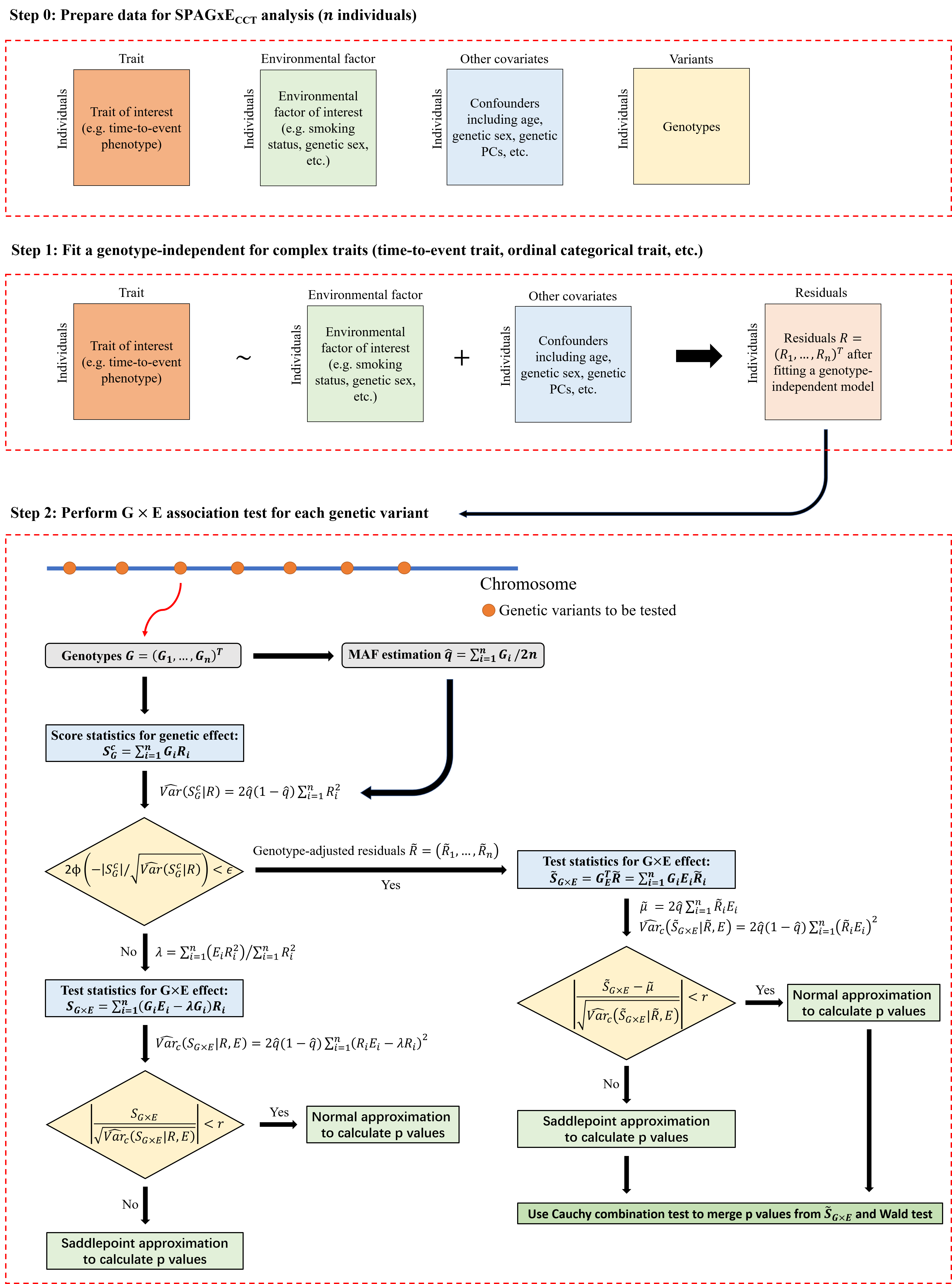
SPAGxECCT is applicable to a wide range of complex traits with intricate structures, including time-to-event, ordinal categorical, binary, quantitative, longitudinal, and other complex traits. The framework involves two main steps:
-
Step 1: SPAGxECCT fits a covariates-only model to calculate model residuals. These covariates include, but are not limited to, confounding factors such as age, sex, SNP-derived principal components (PCs), and environmental factors. The specifics of the model and residuals vary depending on the trait type. Since the covariates-only model is genotype-independent, it only needs to be fitted once across a genome-wide analysis.
-
Step 2: SPAGxECCT identifies genetic variants with marginal G×E effects on the trait of interest. First, marginal genetic effects are tested using score statistics. If the marginal genetic effect is not significant, SG×E is used as the test statistic to characterize the marginal G×E effect. If significant, SG×E is updated to genotype-adjusted test statistics. To balance computational efficiency and accuracy, SPAGxECCT employs a hybrid strategy combining normal distribution approximation and saddlepoint approximation (SPA) to calculate p-values, as used in previous studies such as SAIGE and SPAGE. For variants with significant marginal genetic effects, SPAGxECCT additionally calculates p value through Wald test and uses Cauchy combination (CCT) to combine p values from Wald test and the proposed genotype-adjusted test statistics.
Quick start-up examples (genotype input using R matrix format)
The following example illustrates how to use SPAGxECCT to analyze a binary trait, with genotype data input provided in the R matrix format.
Step 1. Read in data and fit a genotype-independent model
library(SPAGxECCT)
# Simulate phenotype and genotype
N = 10000                                        # sample size
nSNP = 100                                       # number of SNPs
MAF = 0.1                                        # minor allele frequency
Geno.mtx = matrix(rbinom(N*nSNP,2,MAF),N,nSNP)   # genotype matrix
# NOTE: The row and column names of genotype matrix are required.
rownames(Geno.mtx) = paste0("IID-",1:N)
colnames(Geno.mtx) = paste0("SNP-",1:nSNP)

# phenotype data
Phen.mtx = data.frame(ID = paste0("IID-",1:N),
                      Y=rbinom(N,1,0.5),
                      Cov1=rnorm(N),
                      Cov2=rbinom(N,1,0.5),
                      E = rnorm(N))

Cova.mtx = Phen.mtx[,c("Cov1","Cov2")]    # covariates dataframe excluding environmental factor E
E = Phen.mtx$E                            # environmental factor E

# fit a genotype-independent model
R = SPA_G_Get_Resid("binary",
                    glm(formula = Y ~ Cov1+Cov2+E, data = Phen.mtx, family = "binomial"),
                    data=Phen.mtx,
                    pIDs=Phen.mtx$ID,
                    gIDs=paste0("IID-",1:N))
Step 2. Conduct a marker-level association study
# calculate p values
binary.res = SPAGxE_CCT(traits = "binary",                       # trait type
                        Geno.mtx = Geno.mtx,                     # genotype matrix
                        R = R,                                   # residuals from genotype-independent model (null model in which marginal genetic effect and GxE effect are 0)
                        E = E,                                   # environmental factor
                        Phen.mtx = Phen.mtx,                     # phenotype dataframe
                        Cova.mtx = Cova.mtx)                     # covariates dataframe excluding environmental factor E

# we recommand using column of 'p.value.spaGxE.CCT.Wald' to associate genotype with binary phenotypes
head(binary.res)
Quick start-up examples (genotype input using PLINK file format)
The following example illustrates how to use SPAGxECCT to analyze a binary trait, with genotype data input provided in PLINK file format.
Step 1. Read in data and fit a genotype-independent model
library(SPAGxECCT)
# Simulate phenotype and genotype
N = 10000 # sample size

# PLINK format for genotype data
GenoFile = system.file("", "GenoMat_SPAGxE.bed", package = "SPAGxECCT")

# phenotype data
Phen.mtx = data.frame(ID = paste0("IID-",1:N),
                      Y=rbinom(N,1,0.5),
                      Cov1=rnorm(N),
                      Cov2=rbinom(N,1,0.5),
                      E = rnorm(N))

Cova.mtx = Phen.mtx[,c("Cov1","Cov2")]    # covariates dataframe excluding environmental factor E
E = Phen.mtx$E                            # environmental factor E

# fit a genotype-independent model
R = SPA_G_Get_Resid("binary",
                    glm(formula = Y ~ Cov1+Cov2+E, data = Phen.mtx, family = "binomial"),
                    data=Phen.mtx,
                    pIDs=Phen.mtx$ID,
                    gIDs=paste0("IID-",1:N))
Step 2. Conduct a marker-level association study
# calculate p values
binary.res = SPAGxE_CCT(traits = "binary",                       # trait type
                        GenoFile = GenoFile,                     # a character of genotype file
                        R = R,                                   # residuals from genotype-independent model (null model in which marginal genetic effect and GxE effect are 0)
                        E = E,                                   # environmental factor
                        Phen.mtx = Phen.mtx,                     # phenotype dataframe
                        Cova.mtx = Cova.mtx)                     # a covariate matrix excluding the environmental factor E


# we recommand using column of 'p.value.spaGxE.CCT.Wald' to associate genotype with binary phenotypes
head(binary.res)
Quick start-up examples (genotype input using BGEN file format)
The following example illustrates how to use SPAGxECCT to analyze a binary trait, with genotype data input provided in BGEN file format.
Step 1. Read in data and fit a genotype-independent model
library(SPAGxECCT)
# Simulate phenotype and genotype
N = 10000

# BGEN format for genotype data
GenoFile = system.file("", "GenoMat_SPAGxE.bgen", package = "SPAGxECCT")
GenoFileIndex = c(system.file("", "GenoMat_SPAGxE.bgen.bgi", package = "SPAGxECCT"),
                  system.file("", "GenoMat_SPAGxE.sample", package = "SPAGxECCT"))

# phenotype data
Phen.mtx = data.frame(ID = paste0("IID-",1:N),
                      Y=rbinom(N,1,0.5),
                      Cov1=rnorm(N),
                      Cov2=rbinom(N,1,0.5),
                      E = rnorm(N))

Cova.mtx = Phen.mtx[,c("Cov1","Cov2")]    # covariates dataframe excluding environmental factor E
E = Phen.mtx$E                            # environmental factor E

# fit a genotype-independent model
R = SPA_G_Get_Resid("binary",
                    glm(formula = Y ~ Cov1+Cov2+E, data = Phen.mtx, family = "binomial"),
                    data=Phen.mtx,
                    pIDs=Phen.mtx$ID,
                    gIDs=paste0("IID-",1:N))
Step 2. Conduct a marker-level association study
# calculate p values
binary.res = SPAGxE_CCT(traits = "binary",                       # trait type
                        GenoFile = GenoFile,                     # a character of genotype file
                        GenoFileIndex = GenoFileIndex,           # additional index file(s) corresponding to GenoFile
                        R = R,                                   # residuals from genotype-independent model (null model in which marginal genetic effect and GxE effect are 0)
                        E = E,                                   # environmental factor
                        Phen.mtx = Phen.mtx,                     # phenotype dataframe
                        Cova.mtx = Cova.mtx)                     # a covariate matrix excluding the environmental factor E


# we recommand using column of 'p.value.spaGxE.CCT.Wald' to associate genotype with binary phenotypes
head(binary.res)
Citation
- A scalable and accurate framework for large-scale genome-wide gene-environment interaction analysis and its application to time-to-event and ordinal categorical traits (to be updated).